Introduction to lamatrix: Combining models

lamatrix enables you to combine Model objects to build more powerful models for your data. This tutorial will show how models can be combined.

import numpy as np
from astropy.io import fits
import matplotlib.pyplot as plt

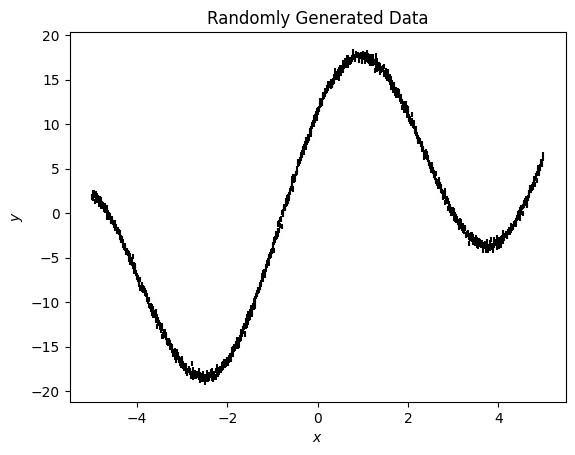
First, we will make some fake data to fit. Here I’m creating data which is a combination of a simple polynomial, a sinusoid, and some noise terms.

x = np.arange(-5, 5, 0.01)
y = x * 2.3459 + 1.435 + np.random.normal(0, 0.3, size=len(x))
ye = np.ones(len(x)) * 0.3

y += 10*np.sin(x) + 10*np.cos(x)

If we plot the data we can see this is a simple trend

fig, ax = plt.subplots()
ax.errorbar(x, y, ye, ls='', c='k')
ax.set(xlabel='$x$', ylabel='$y$', title='Randomly Generated Data');

Now we will use lamatrix to fit this data.

from lamatrix import Polynomial, Sinusoid, Constant

In this case, we know our model is a linear combination of these trends, so we simply add them together. Note we know both the polynomial and sinusoid are functions of the same variable, which we name "x".

model = Polynomial('x', order=1) + Sinusoid('x') + Constant()

model

JointModel
        Polynomial(x)[n, 1]
        Sinusoid(x)[n, 2]
        Constant()[n, 1]

The model is now a JointModel where there are multiple components

We’ve combined different models, but we are still able to use it in the same way as a simple model. For example, here’s the equation for the model

model.equation

\[f(\mathbf{x}) = w_{0} \mathbf{x}^{1} + w_{1} \sin(\mathbf{x}) + w_{2} \cos(\mathbf{x}) + w_{3} \]

Now we have the model, we can simply use the fit class method.

model.fit(x=x, data=y, errors=ye)

The model fit with no errors, let’s look at the posterior distributions.

model.posteriors

DistributionContainer
        [(2.3465, 0.0034), (10.008, 0.013), (10.016, 0.014), (1.4568, 0.0099)]

We can see we’ve fit the posteriors with small errors. Let’s compare to our inputs. Our input polynomial was

\(2.3459x + 1.435\)

Because model is a linear combination of objects, we can split this model back into it’s components:

model

JointModel
        Polynomial(x)[n, 1]
        Sinusoid(x)[n, 2]
        Constant()[n, 1]

model[0]

Polynomial(x)[n, 1]

model[0].posteriors

DistributionContainer
        [(2.3465, 0.0034)]

We can see that the first order polynomial has posteriors after our fit. This is only a first order polynomial, and so it has only one weight. The weight is very close to our input weight of 2.346!

The polynomial we used was \(10.sin(x) + 10.cos(x)\). Let’s look at the posteriors.

model[1]

Sinusoid(x)[n, 2]

model[1].equation

\[f(\mathbf{x}) = w_{0} \sin(\mathbf{x}) + w_{1} \cos(\mathbf{x})\]

model[1].posteriors

DistributionContainer
        [(10.008, 0.013), (10.016, 0.014)]

This has two weights, one for sine and one for cosine. The weights are very close to the input amplitudes!

Finally we have the constant term

model[2]

Constant()[n, 1]

model[2].posteriors

DistributionContainer
        [(1.4568, 0.0099)]

This is very close to our input offset term. Let’s plot the model to see how this looks

fig, ax = plt.subplots()
ax.errorbar(x, y, ye, ls='', c='k')
ax.plot(x, np.asarray([model.sample(x=x) for count in range(100)]).T, c='r', alpha=0.1);
ax.set(xlabel='$x$', ylabel='$y$', title='Randomly Generated Data');

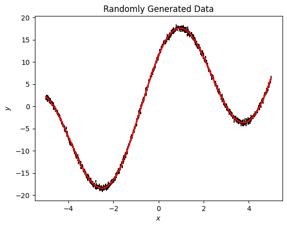
This is a great fit to the data!

Here we’ve combined two types of model, a sinusoid and a polynomial, in order to fit the data we have. In this case, we knew the form of the models we should use. We can combine any number and any type of models in this way.

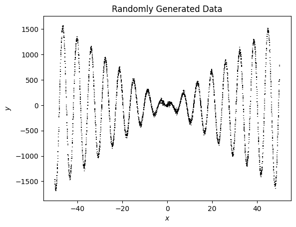
In this case we’ve fit a model where the two components are added, let’s try a model where they are multiplied.

x = np.arange(-50, 50, 0.01)
y = x * 2.3459 + np.random.normal(0, 2, size=len(x))
ye = np.ones(len(x)) * 2

y *= 10*np.sin(x) + 10*np.cos(x)
y += 1.435

fig, ax = plt.subplots()
ax.errorbar(x, y, ye, ls='', c='k')
ax.set(xlabel='$x$', ylabel='$y$', title='Randomly Generated Data');

Now we need to multiply some components of the model

model = (Polynomial('x', order=3) * Sinusoid('x')) + Constant()

The model is now a JointModel, but inside the model is a CrossTermModel

model

JointModel
        CrosstermModel(x)[n, 6]
        Constant()[n, 1]

This crossterm model is the Polynomial multiplied by the Sinusoid

model[0]

CrosstermModel(x)[n, 6]

This model is now a polynomial multiplied by a sinusoid. Let’s look at the equation

model[0].equation

\[f(\mathbf{x}) = w_{0} \mathbf{x}^{1}\sin(\mathbf{x}) + w_{1} \mathbf{x}^{1}\cos(\mathbf{x}) + w_{2} \mathbf{x}^{2}\sin(\mathbf{x}) + w_{3} \mathbf{x}^{2}\cos(\mathbf{x}) + w_{4} \mathbf{x}^{3}\sin(\mathbf{x}) + w_{5} \mathbf{x}^{3}\cos(\mathbf{x})\]

We see in this model each term of the sinusoid model is multiplied by each term of the polynomial model. Note that a CrosstermModel can not be indexed into, because we can not split apart the various components.

We can fit this model just like the one above to find the best fitting components

model.fit(x=x, data=y, errors=ye)

fig, ax = plt.subplots()
ax.errorbar(x, y, ye, ls='', c='k')
ax.plot(x, np.asarray([model.sample(x=x) for count in range(100)]).T, c='r', alpha=0.1);
ax.set(xlabel='$x$', ylabel='$y$', title='Randomly Generated Data');

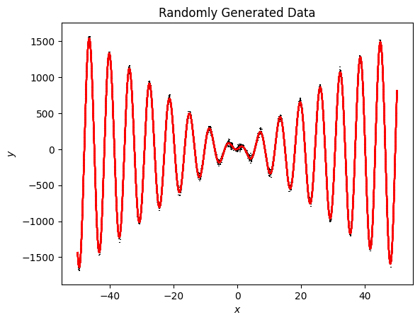
This let’s us find the best fitting weights for our combined model

model.posteriors

DistributionContainer
        [(23.4143, 0.0024), (23.4681, 0.0025), (0.000125, 2.5e-05), (0.000271, 2.6e-05), (2.64e-05, 1.5e-06), (-5.3e-06, 1.5e-06), (1.547, 0.02)]

We can save and load joint and crossterm models just like regular models

model.save("output.json")

from lamatrix import load

load("output.json")

JointModel
        CrosstermModel(x)[n, 6]
        Constant()[n, 1]